So, what is the operation time of an electromechanical relay for a given arcing current? To do this you will need the following information.

1. Ratio of current transformers.
2. The current rating of the relay.
3. The time / PSM curve of the relay.
4. The time multiplier setting.
5. The plug setting multiplier position.

The current transformer (CT) ratio (a) is covered in an earlier section, just make sure that the current rating of the relay (b) matches the secondary of the CT. The relay current rating can usually be found on the front of the relay cover as shown in Figure 8.4. The time/PSM curve (c) is usually provided on the relay cover as well as in manufacturer’s literature. If the source of the information is the latter, it may be presented as the characteristic curve shown in Figure 8.6. The time multiplier setting (d) and the plug setting multiplier position (e) can be taken directly from the relay, as shown in Figure 8.4.

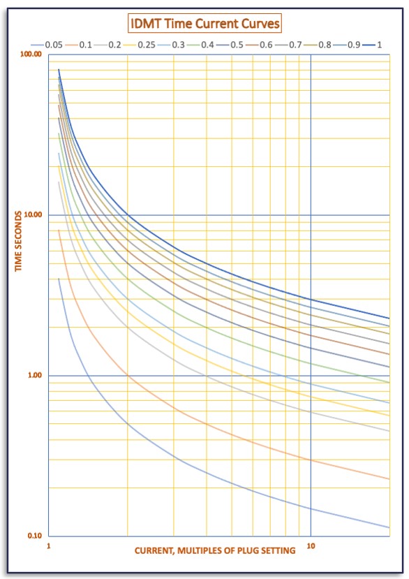
Figure 8.6

As an example, if we have the following information, we can determine the relay time to operate; CT ratio = 400/5, current rating of the relay = 5A, the curve is shown in Figure 8.4 above, the time multiplier setting TMS = 0.2 and the plug setting multiplier position is 100%. We have calculated an arcing fault current of I_arc = 5000 amperes.

Bear in mind that there is the time for the circuit breaker to operate to take into account as well as relay inaccuracies. Both these factors need to be added to the relay trip time before applying this to calculate the incident energy. Some further information to follow.

Warning - Never touch the moving parts of electromagnetic IDMT relays. Actions such as in trying to manually turn the disc or bending contacts can warp moving parts or introduce acidity which may result in decay to contact surfaces.

8.4.3 Static Relays

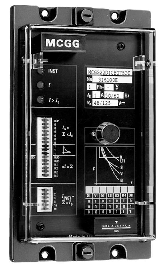
Figure 8.7 Static Relay

Static Relays were first introduced the 1960s and gained in popularity in the 1970s. They were the next generation on from induction disc electromechanical types. So called static relays meant that they have no moving mechanical parts and monitored the voltage and current incoming waveforms by analogue circuits.

They were an electronic replacement for electromechanical relays designed to carry out the same functions but performed better as they are more accurate, are fast acting and caused less burden on current transformers. Knowledge of electromechanical IDMT relays meant that settings and, in this case, data collection is fairly straightforward. The static relay shown in Figure 8.7 was a very popular model which arrow switches to select and set the required time current characteristic shown on the front panel. This same format was adopted by several manufacturers. For data collection, this makes the process fairly straightforward as all the information is on display. Most user manuals are easy to obtain by google even if some of the relays are over thirty years old. Manufacturers are keen to make information accessible, even about obsolete products so no need to pay specialist companies for photocopied documents.